


Home → How-to Guides → Solution Examples → Architecture Examples → PID Process Trainer AI Designer Example
This example demonstrates the solution PIDProcessTrainer created by FrameworX AI Designer — a fired heater with three live control loops you can tune, disturb, and measure.
Solution download: PIDProcessTrainer.dbsln
Showcases:
- PID control running as a real closed loop, four times per second.
- Cascade control — one loop commanding another.
- Open-loop step testing with automatic model identification and three tuning methods.
- Loop performance measurement: overshoot, settling time, IAE, valve travel.
- Process graphics, faceplates, trends, and alarms on one screen set.
The downloadable solution requires FrameworX 10.1.5d or later. It will not open on earlier versions.
What the solution does
The solution simulates the feed section of a fired heater — the kind found in a refinery or petrochemical plant. Oil is pumped from a feed tank through a furnace and leaves at a controlled temperature.
Three control loops run continuously:
Loop | Controls | Character |
|---|---|---|
LIC-101 | Feed tank level | Integrating process — level keeps moving until inflow and outflow match |
FIC-101 | Fuel gas flow to the burners | Fast and noisy, typical of a flow loop |
TIC-101 | Heater outlet temperature | Slow, with 22 seconds of dead time before the temperature reacts |
TIC-101 and FIC-101 run in cascade. The temperature loop does not move the fuel valve directly — it asks the flow loop for a fuel rate, and the flow loop delivers exactly that. This is standard practice on fired heaters, and the example shows it working end to end.
Everything the loops respond to comes from a process model running inside the solution, so the behaviour is repeatable: the same starting point and the same actions reproduce the same result every time. That makes before-and-after comparisons meaningful when you change a tuning parameter.
The screens
Unit overview
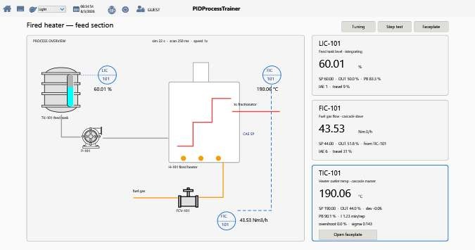
The process drawing, with live values and standard instrument symbols. The dashed line between TIC-101 and FIC-101 shows the cascade. Cards on the right summarise each loop — measured value, setpoint, output, and the tuning currently in force.
Loop tuning
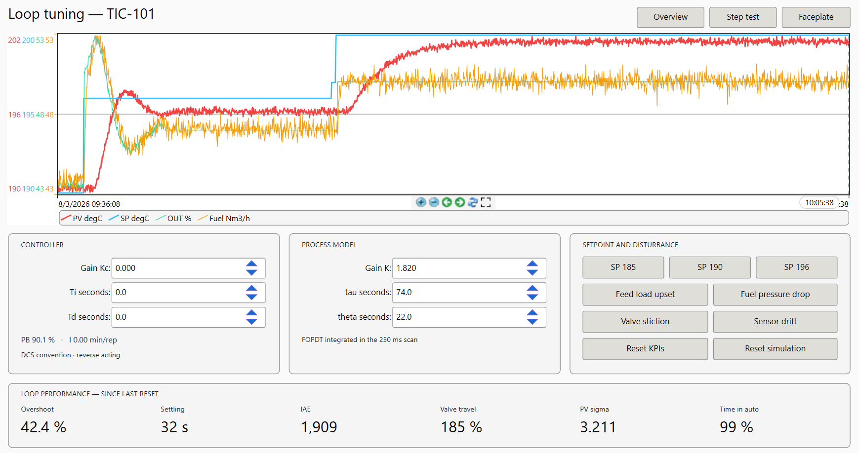
The screen to spend time on. The trend at the top shows the measured temperature, the setpoint, the controller output, and the fuel gas flow together. Below it you can change the controller tuning, change the process itself, and inject disturbances — then watch what each change does.
The tiles across the bottom score the result: overshoot, settling time, IAE, valve travel, measurement variability, and time in automatic. Valve travel and variability are the numbers a plant actually reports on, because excessive valve movement wears equipment out.
Step test and auto-tune
Answers the question every engineer asks: what tuning numbers should I use?
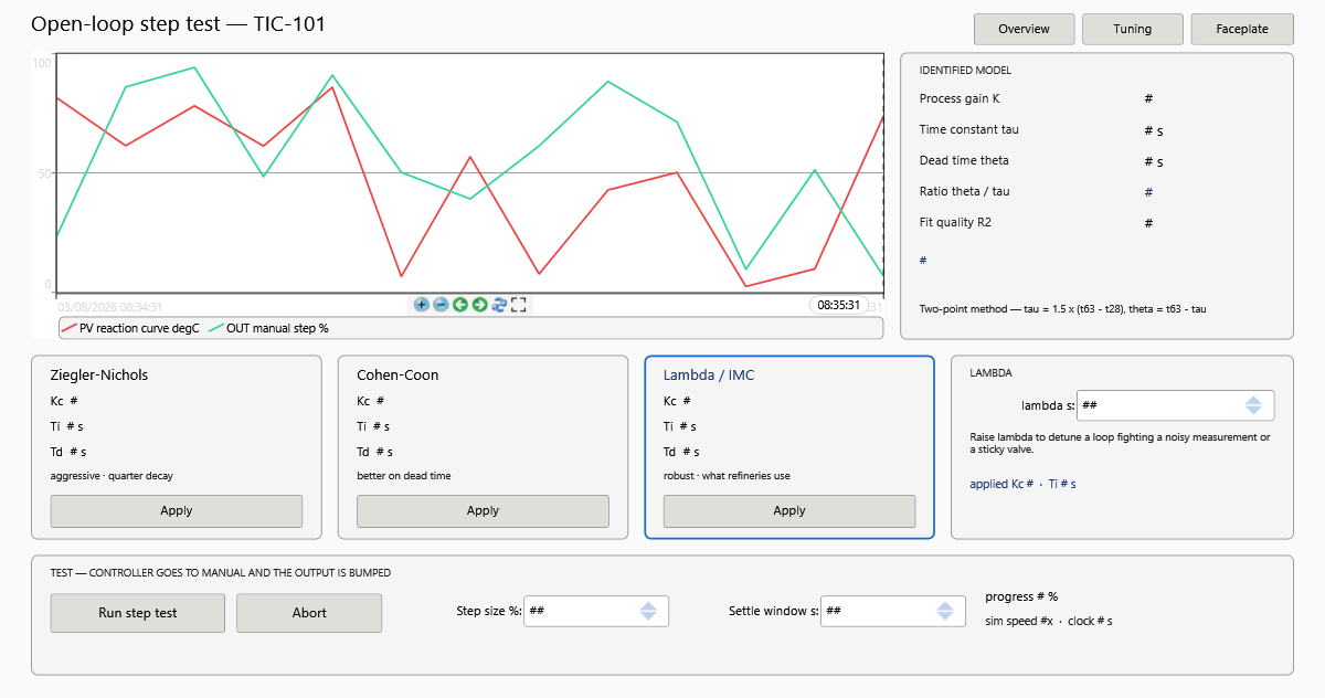
The controller is put into manual, the output is bumped by a fixed amount, and the response is recorded. From that curve the solution identifies the three characteristics of the process — how strongly it responds, how quickly, and how long it waits before reacting — then calculates tuning by three established methods: Ziegler-Nichols, Cohen-Coon, and Lambda (IMC). One click applies any of them to the live controller.
Loop faceplate
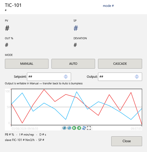
The pop-up an operator uses: measured value, setpoint, output and deviation, with Manual / Automatic / Cascade selection, setpoint and output entry, and a short trend. Switching from Manual back to Automatic is bumpless — the output does not jump.
Try it yourself
- Open the solution and start the runtime. The heater settles at 190 °C.
- Go to Loop tuning and press SP 196. Watch the temperature climb to the new setpoint through the dead time.
- Press Fuel pressure drop. The fuel supply weakens — watch the cascade correct it before the temperature moves much.
- Press Reset KPIs, change the controller gain, and repeat the setpoint step. Compare the scores.
- Go to Step test, press Run step test, and let it finish. Apply the Lambda tuning and step the setpoint again.
How the control is built
The PID algorithm and the process model are written in C# as reusable script classes inside the solution. One implementation serves all three loops — define the controller once, then create as many loops as the plant needs. Because it is ordinary code, the behaviour is fully visible and adjustable: the controller in this example uses the standard ISA form with anti-windup, bumpless transfer, and derivative acting on the measurement.
The process graphics are drawn on a standard display canvas using the built-in symbol library — tanks, pumps, valves and instrument bubbles — so a screen like the unit overview is assembled rather than coded. Trends, alarms and historical logging are configured, not programmed: the deviation and saturation alarms on this example are ordinary alarm entries, and every pen on every trend is a logged value.
The controller tuning is exposed in both conventions engineers use — gain and seconds, or proportional band and minutes per repeat — so the numbers on the faceplate match what a DCS would show.
Related
Data Calculation and Processing Code — code library snippets for process calculations.
Scripts Tasks and Classes Example — how script tasks and classes are structured.